Preset guide

Everything this app draws comes from a preset: a small TOML file that names one built-in rendering system and binds that system’s parameters to short expressions over the live audio analysis. No Rust, no shaders, no rebuild — you edit a line, save, and the running window picks it up within about 150 ms.

This is the entrance. It shows you what the built-in systems look like, which of the three reference documents owns which surface, and the loop you actually work in. It deliberately reproduces no table from those references: where you need a parameter, a function or a palette name, this page says which document owns it and links there (ADR-0101).

Where to go from here:

You want	Go to
The parameter reference: every parameter, its default, its range, what it does	Parameter roster
The expression grammar — variables, functions, operators	Expression language
Palettes, custom stops, the A/B crossfade	Colour and palettes
One preset tuned step by step, with the numbers	Tuning walkthrough

Every picture on this page is a headless render of the engine, captured by the shot CLI under a synthesized audio clip — not a screenshot of the application window. They are regenerated by node scripts/docs-shots.mjs, whose manifest records the preset, stimulus, hop, size and tier behind each one (ADR-0100).

---

1. A preset in ten lines

This is a complete, working preset. It is docs/examples/minimal.toml, and the picture below it is that exact file rendered:

system = "parametric_curve"
name = "Ten Lines"

[curve]
family = "maurer_rose"

[params]
n          = "6"
scale      = "0.55 + clamp(bass * 0.35, 0, 0.30)"
brightness = "0.80 + clamp(mid * 0.45, 0, 0.40)"
hue        = "0.55 + time * 0.02"

Four things are worth naming, because they are the whole model:

• system picks what gets drawn. One of a closed list of names, in section 2. Everything else in the file is interpreted against that choice — n means something to a parametric_curve and nothing at all to a swarm.
• [params] values are expressions, not numbers. Each one is re-evaluated every frame against the current analysis. "6" is a constant that happens to be written as an expression; the other three move.
• bass, mid, time are the vocabulary. There is more of it — beat, bar, onset, tempo, counters, a 64-band spectrum accessor — and Expression language is the reference.
• clamp(x, lo, hi) is doing the real work. bass * 0.35 is a gain: it decides how much of the music reaches the parameter. The clamp is a limit: it decides how far the parameter is allowed to travel. Getting the gain wrong is the single most common way a preset ends up looking dead, and step 3 of the walkthrough is about exactly that.

Some systems also take a structural table — [curve] here, [generator] for the two generator systems, [particles] for the attractor, [spectrum] for the readout, [field] for the analytic field, [cellular] for the automaton, [plexus] for the network, [voxel] for the 3D automaton. Those are declarative configuration read once when the preset loads, not expressions: they choose which figure, and the params then animate it.

---

2. The systems

One image each, captured under the same stimulus at the same moment in the clip, so they are comparable. Each is a real preset, and the file name is under the picture: a presets/ name is a shipped preset, while a docs/examples/ name is a teaching preset, written to show one family plainly and never shipped. A family no shipped preset draws yet is pictured through one of those. The parameter reference — every parameter of every system, with its default, the range that reads and what it does — is Parameter roster.

fragment_field

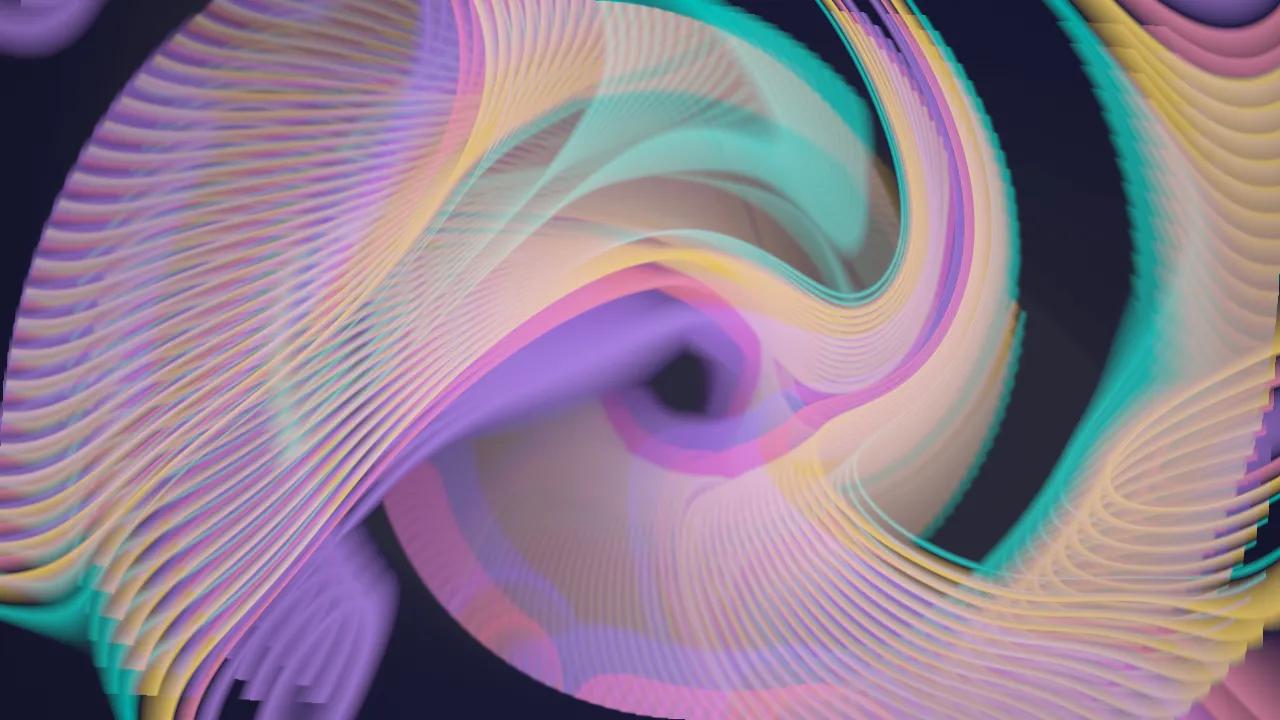
presets/fragment_whorl.toml

A fullscreen shader. Every pixel is computed from a domain-warped noise field and coloured through the shared palette, so there is no geometry and no particle count — the whole frame is the subject. It is the cheapest system to make busy and the hardest to make sparse.

Reach for this when you want an edge-to-edge look with no figure in it: auroras, marbling, plasma, oil-on-water.

swarm

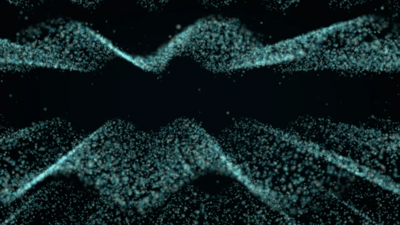
presets/swarm_braid.toml

Around ten thousand CPU-simulated particles drifting through a flow field in a volume, seen through a perspective camera and drawn as additive marks. Near marks draw larger and cross the screen faster than far ones, and a focal plane can keep one layer sharp while the layers in front and behind soften. Their world wraps, so nothing ever leaves the frame — the field stays populated without respawn hitches.

Reach for this when the look is a motion: murmuration, drift, a shoal turning. Be warned that this is the system a still photograph serves worst, for exactly that reason.

parametric_curve

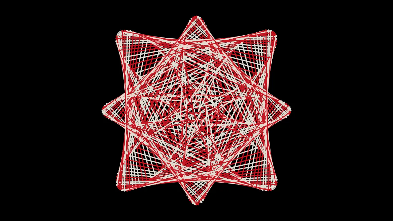
presets/curve_broadside.toml

One continuous line, sampled every frame from a closed-form t → (x, y) curve and drawn as thick glowing strokes. Because it is resampled per frame rather than cached, audio can sweep the shape itself, not just its colour and scale.

Reach for this when you want precise line art whose geometry is the reaction.

The picture above is the Maurer rose, one of seven curve families a [curve] family line picks between: five flat ones and two that live in space. Five more are below, each rendered from a small teaching preset — the file under the picture is the whole recipe. What n, d and phase mean on each family, and which levers belong to which, is the [curve] table in the grammar reference.

family = "lissajous" — docs/examples/curves/lissajous.toml

Two sine waves at right angles, one per axis. Whole frequencies close the figure; a fractional one leaves it open and drifting.

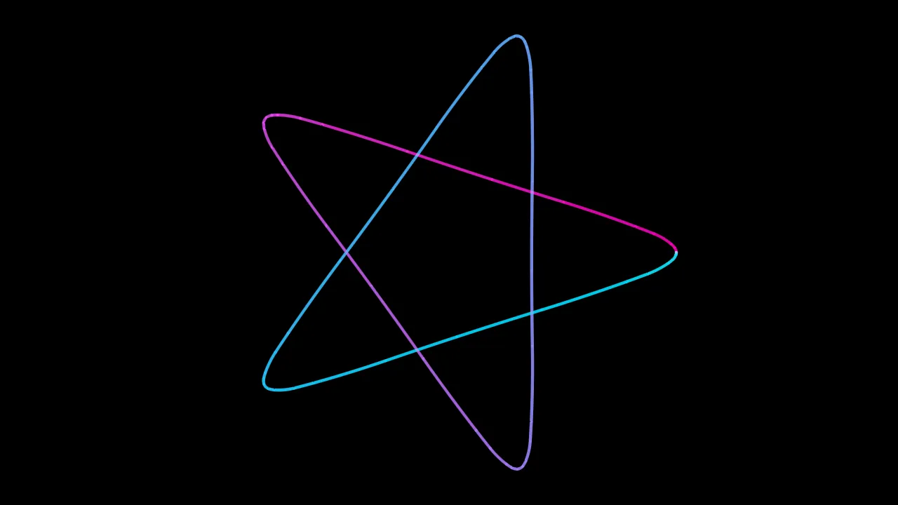
family = "hypotrochoid" — docs/examples/curves/hypotrochoid.toml

The spirograph: a circle rolling inside a fixed one, traced by a pen. pen moves the pen from rounded loops through sharp cusps to overlapping petals, and a negative n rolls the circle outside.

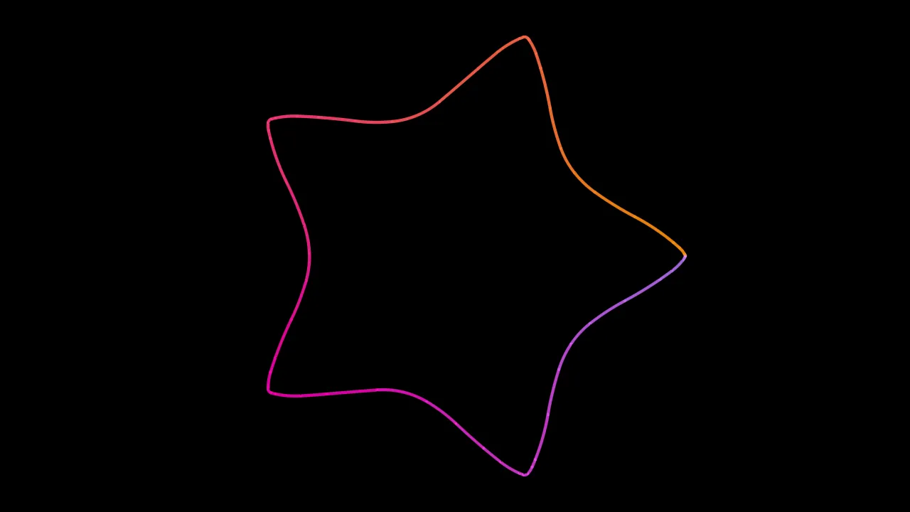
family = "superformula" — docs/examples/curves/superformula.toml

Starfish, flowers, polygons and rounded shells from four numbers. sym is a whole count of lobes, which makes it the family that most rewards a [hold] on the bar.

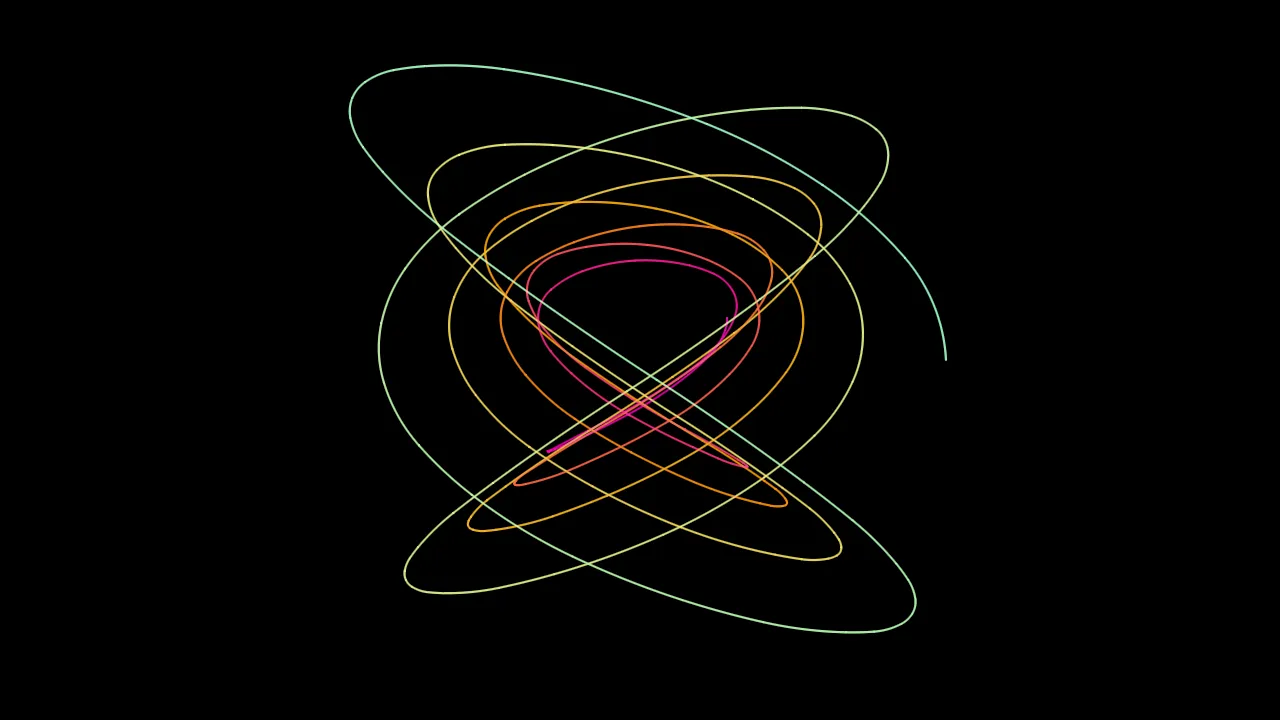
family = "harmonograph" — docs/examples/curves/harmonograph.toml

Two damped pendulums: a Lissajous figure whose swing dies away along the trace, so it spirals inward rather than closing. It is the family that best rewards draw_progress, which draws the trace on from the outside in.

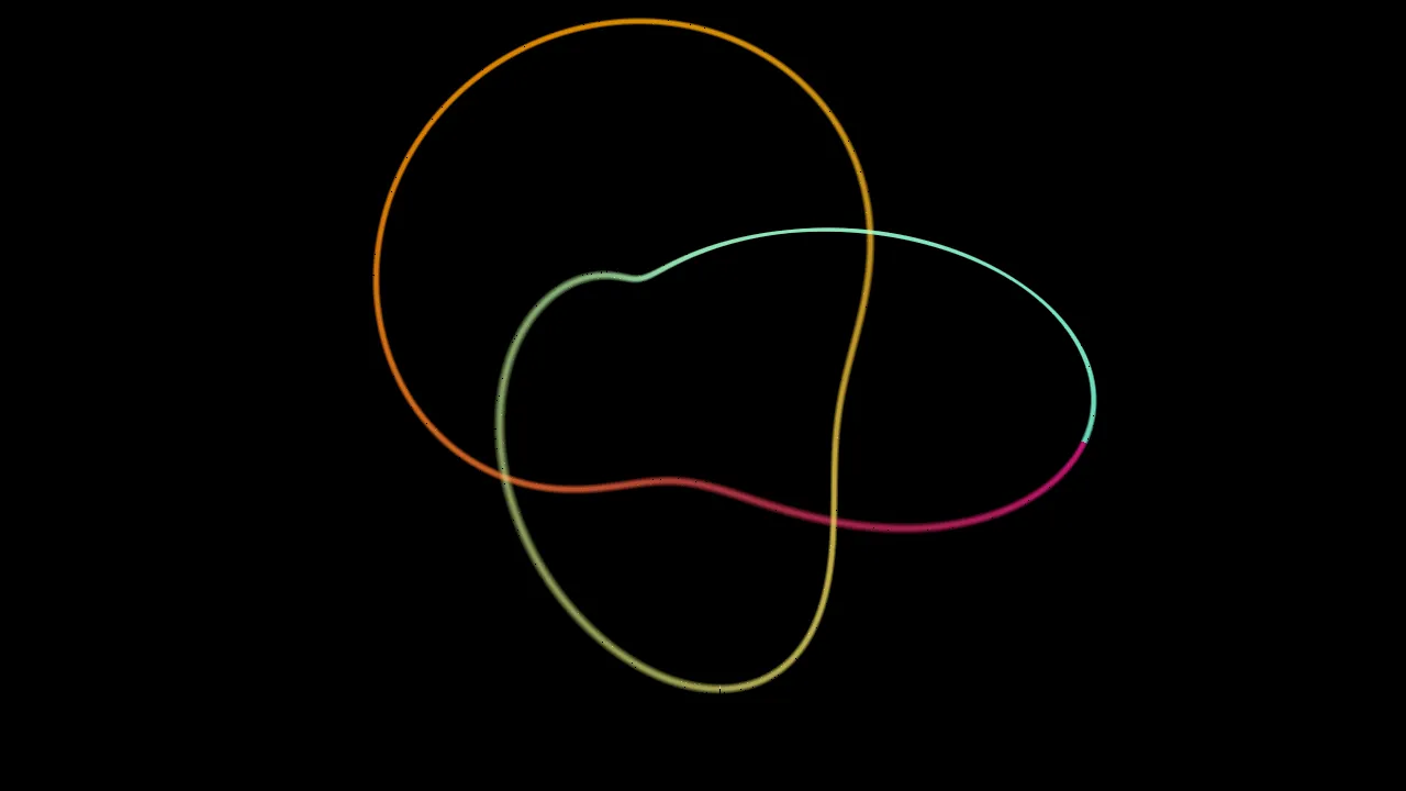
family = "torus_knot" — docs/examples/curves/torus_knot.toml

A strand wound round a doughnut, drawn in three dimensions and seen through a camera. yaw, pitch and distance place that camera, so a slow clock on yaw orbits the knot, and focus with aperture blur the strand away from a focal plane. Its sibling lissajous_3d adds a depth axis to the Lissajous figure. mirror_order, mirror_reflect, spin and stroke_blend belong to the flat families and do nothing on these two.

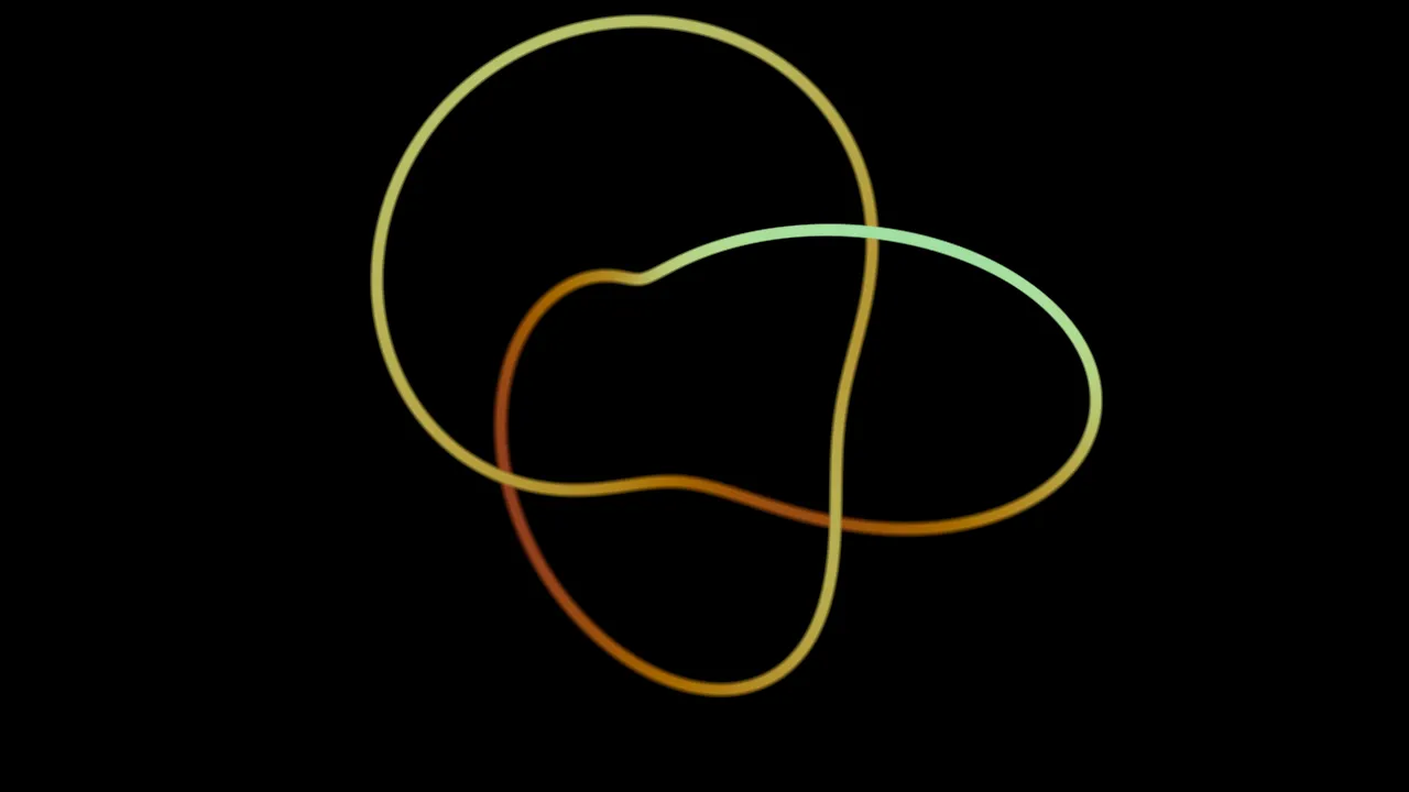
solid, fog and hue_axis — docs/examples/curves/torus_knot_solid.toml

By default the strand is light, and where it crosses itself the crossing glows. solid = "1" paints the near loops over the far ones instead, so the knot reads as an object, and fog darkens the far side. hue_axis = "1" colours the strand by depth rather than along its length. The same solid and fog work on plexus and waterfall; what each costs is in the [plexus] table.

lsystem

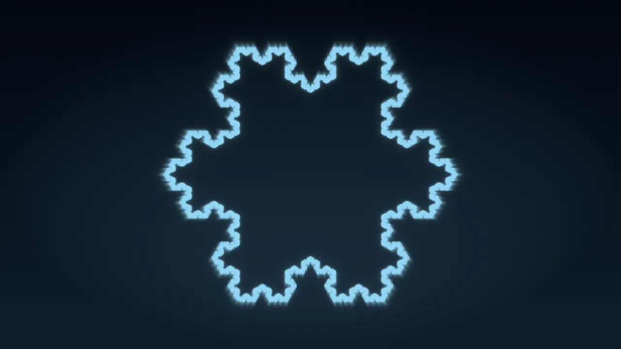
presets/lsystem_rime.toml

A turtle walking a string produced by rewriting an axiom with production rules. The expansion happens once when the preset loads — one cached segment buffer per depth — so per frame the scene only picks a visible depth and transforms it.

Reach for this when you want structure that grows: branching, botanical, or space-filling figures, and a draw_progress that traces them on.

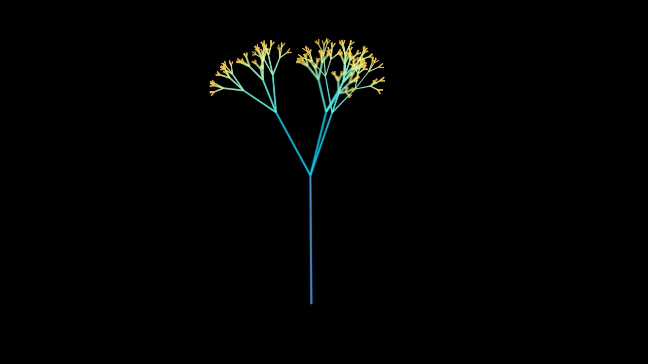
turtle = "space" — docs/examples/lsystem/space_tree.toml

turtle = "space" walks the grammar in depth: & and ^ pitch, \ and / roll, and | turns the turtle around. The tree is seen through the same camera block as the space curves, so aperture softens the branches away from the focal plane.

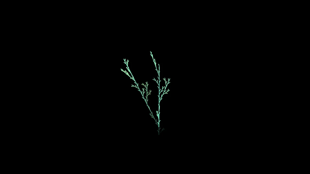
growth = "endless" — docs/examples/lsystem/endless_vine.toml

growth = "endless" grows a vine that never ends. It grows at the rate grow sets and keeps the newest trail segments, fading the oldest, and the view follows the growing tip. Vines and short-branched grammars suit it; the keys are in the [generator] table.

star_pattern

presets/star_rosewindow.toml

A Hankin star rosette built by the contact-angle method — n contact points on a circle, rays leaving at a continuous contact angle, meeting at the petal tips. The rosette is cached and cheap to animate, and the contact angle is a continuous parameter, so the interlacing can open and close.

Reach for this when you want hard radial geometry: rose windows, Islamic star patterns, mandalas with real construction behind them.

reaction_diffusion

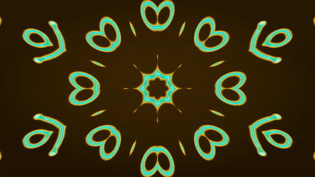
presets/reaction_verdigris.toml

A Gray-Scott simulation stepped on a ping-pong texture pair. It is stateful: each frame’s field depends on the last one, which is what produces the restructuring, growing, organic look that stateless scenes cannot.

Reach for this when you want pattern that evolves rather than animates — spots, stripes, coral, tissue.

attractor

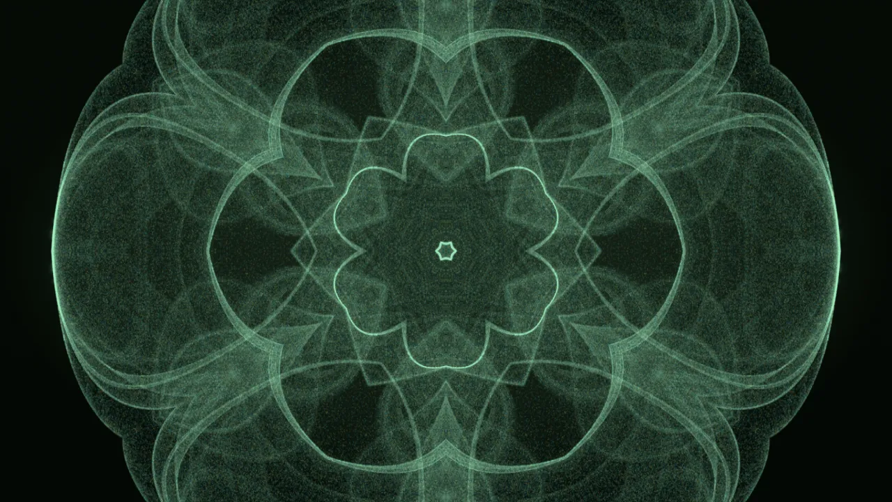
presets/attractor_leviathan.toml

A very large number of points iterated through a chaotic map or an IFS and deposited into an accumulating trail buffer that fades. The figure is not drawn so much as exposed: it builds up over seconds, so this is the family that most rewards a late capture.

Reach for this when you want fine filamentary structure — smoke, ink, dust, strange-attractor figures. It has by far the largest parameter surface, and much of it is family-specific.

spectrum

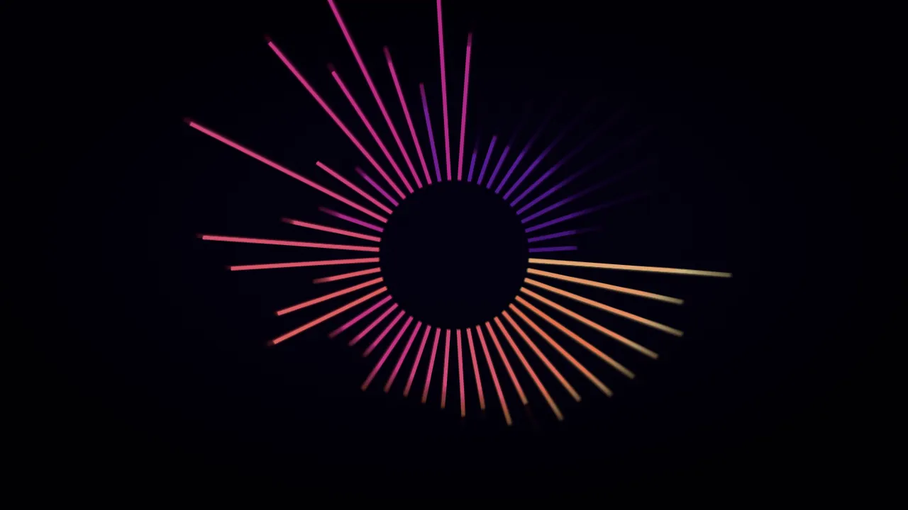
presets/spectrum_radialbloom.toml

A direct readout of the analysis frame’s 64-band log-spaced spectrum, drawn as bars, a polyline or a radial ring of spokes. It is the one system where the audio is literally legible in the picture.

Reach for this when you want the music visible as data rather than as an impression. Note that this system cannot be verified with --set — that path leaves the band array silent, so the readout renders as its inert resting comb; use --signal or --audio.

emitter

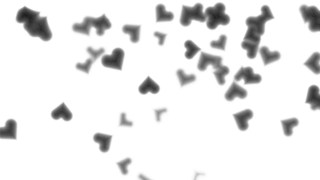
presets/emitter_heartfall.toml

Objects that spawn, follow an analytic ballistic path, age, and are retired. It is the only system whose population is not fixed — which is precisely what the swarm’s wrap-around torus cannot express.

Reach for this when the look is made of discrete events: fireworks, meteors, sparks, anything that should be triggered by a beat rather than modulated by a band.

shape_field

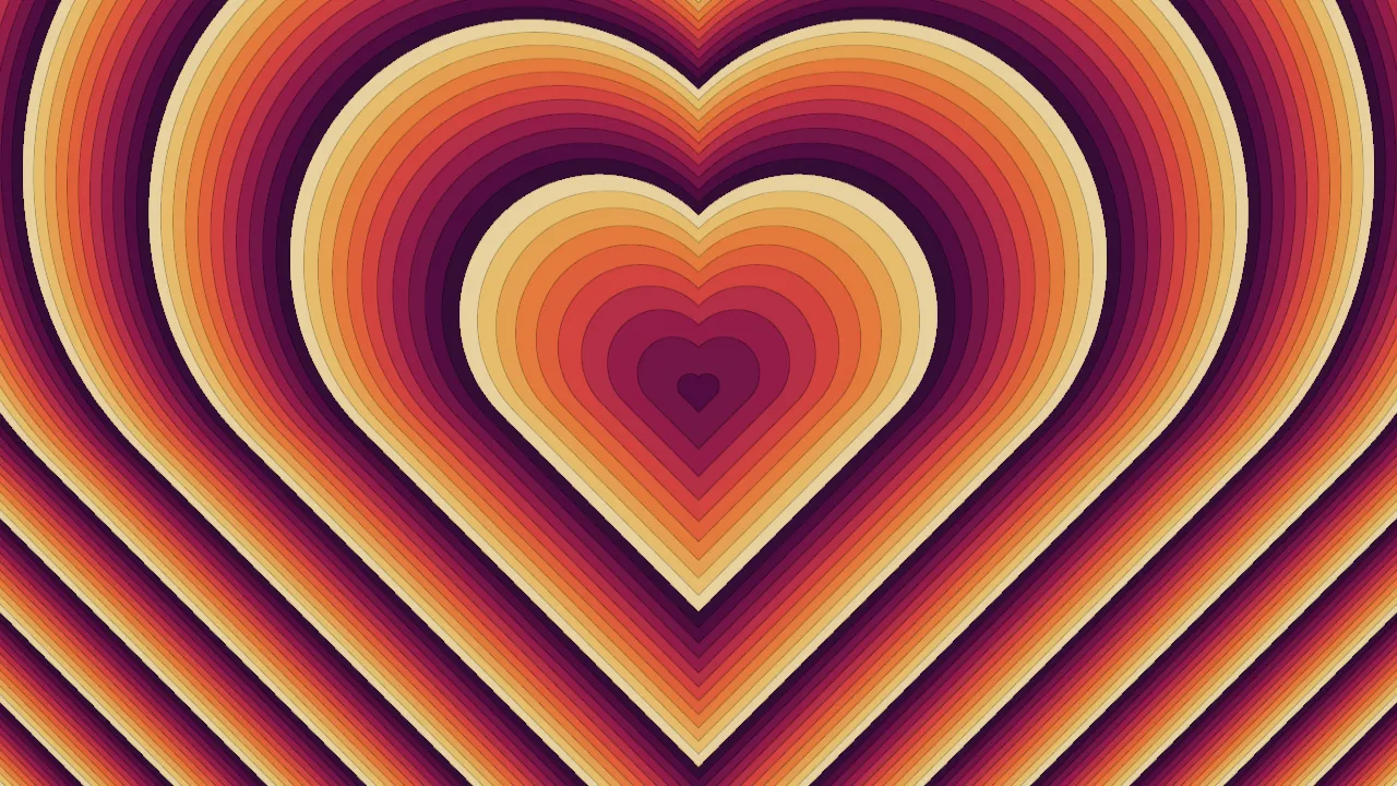
presets/shape_strataheart.toml

It draws one of five silhouettes — disc, ring, polygon, star, heart — as a fullscreen distance field, which makes the palette coordinate a distance: turn palette_steps up and you get concentric offset contours of that shape, not concentric circles. palette_contour then draws a hairline at each band edge.

It is also the one system where the figure itself can be authored rather than selected. A [path] table takes inline SVG path data — one closed contour, pasted out of a design tool and rendered as the same distance field, so palette_steps and palette_contour band an outline nobody put in the roster. presets/shape_maple.toml is that: a maple leaf, 54 commands. A second contour in morph_to gives the bindable morph, so a figure can become another figure on the beat.

Reach for this when the subject is a figure and its echoes: nested outlines, a breathing heart, rings travelling outward from a shape — or one specific emblem the five names do not reach. The full parameter roster, the [path] subset and its arity ceiling, and three worked reactivity recipes are in Parameter roster.

warp_mesh

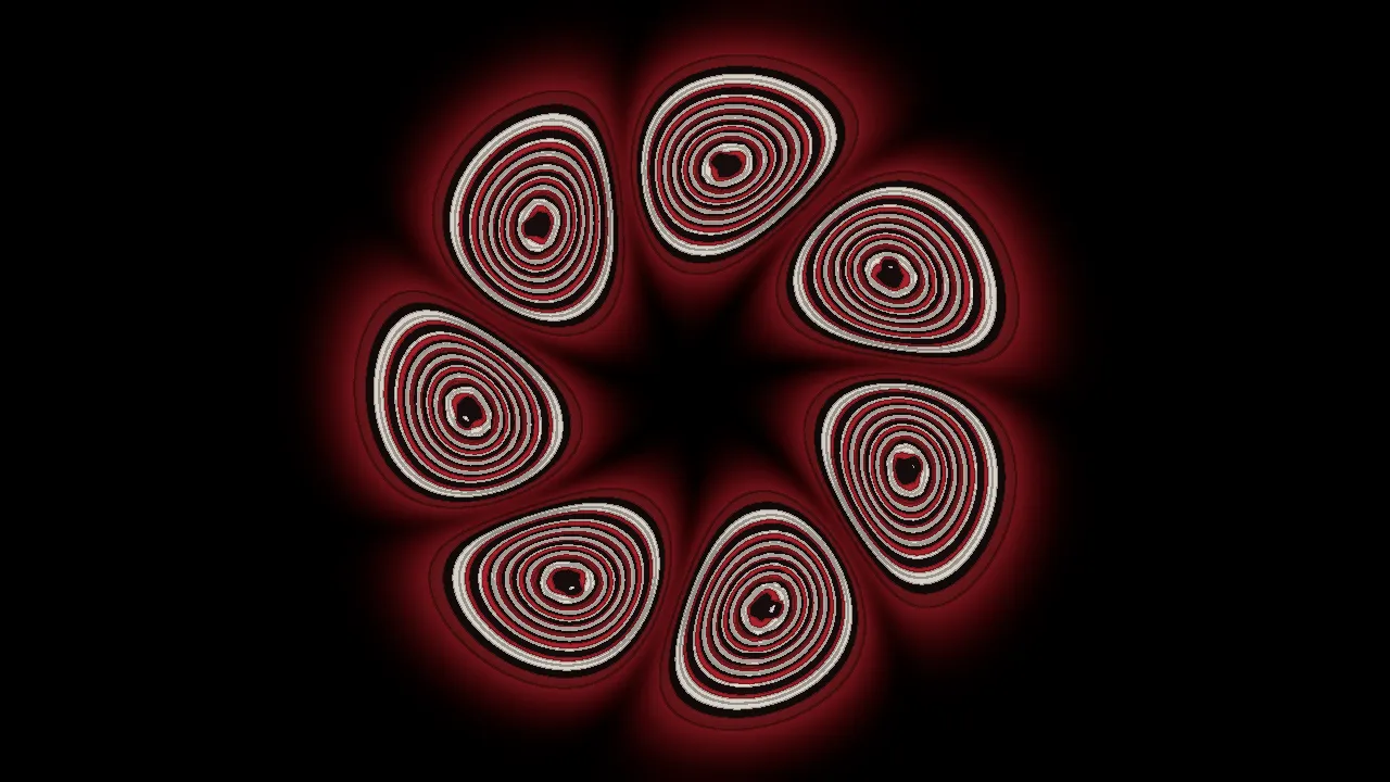
presets/warp_tracery.toml

It covers the frame with a grid of cells and resamples the previous frame through it, giving every grid vertex its own zoom, rotation, stretch and drift — so the past can spiral in one corner and drift in another, which no single whole-frame fb_* transform can express. It is also the only scene with nothing of its own to draw: turn the deposit off and the frame goes black in about a second.

Reach for this when the subject is the history of the image rather than a figure in it: tunnels, vortices, anything where what you are looking at is where the last frame went. A converted MilkDrop preset brings its own draw layer and is the exception; see the [milk] table in Parameter roster.

shape_collage

presets/collage_suprematist.toml

It is the engine’s only graphic world rather than a luminous one. Every other system emits additive light, which has no notion of one object being in front of another — a black bar over a red one simply adds. This one paints: each pixel starts at the paper colour and walks an array of flat elements in array order, compositing each with over, so the array index is the depth. There is no glow, no bloom and no soft edge, and that is the vocabulary rather than an omission.

Reach for this when the look is flat colour and hard edges on a light ground: suprematist and constructivist canvases, poster shapes, anything where solid opaque forms overlap. The one authoring fact is that the palette stays under linear 0.6 — see Colour and palettes.

analytic_field

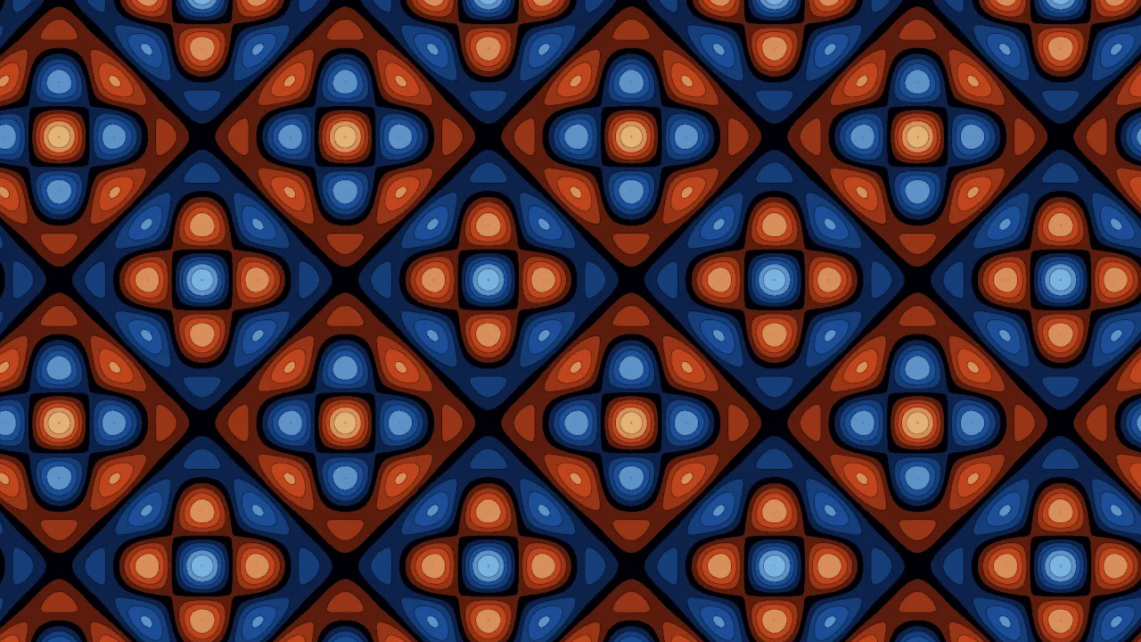
family = "chladni" — presets/analytic_standingwave.toml; the teaching preset is docs/examples/field/chladni.toml

One fullscreen pass that computes a closed-form function of position — no state, no geometry, nothing accumulated, so every frame is exactly what this frame’s bindings say. A [field] family line picks which function, and each family is a whole mathematical world with its own parameters.

The picture above is the Chladni plate: the lines where sand settles on a vibrating square plate, for two whole mode numbers. Change a mode and the whole figure re-forms, so the family most rewards a [hold] on the bar — the example holds its second mode that way, stepping it with the bass.

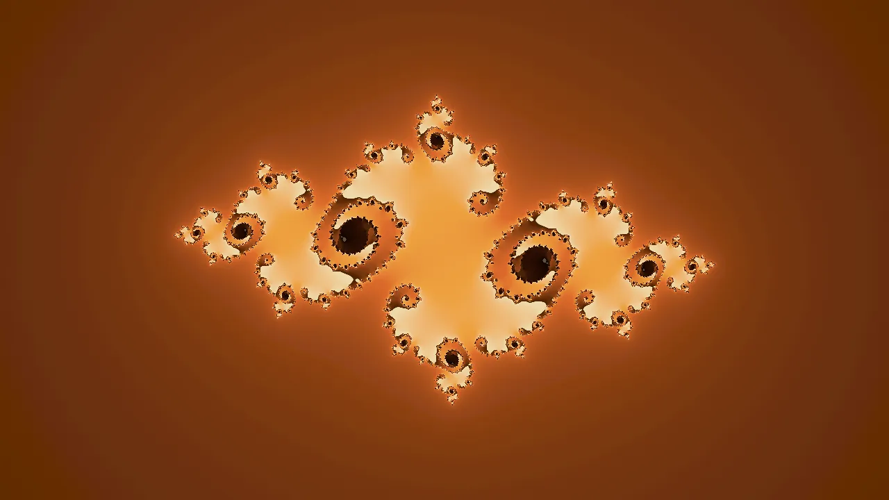
family = "escape_time" — docs/examples/field/escape_time.toml

Escape time: the Julia and Mandelbrot sets, coloured by a smooth count so the boundary glows rather than bands. On a Julia set the constant c is the lever — the bass here nudges it — and carrying it outside the Mandelbrot set breaks the figure into dust. An orbit trap recolours the set by how near each point’s orbit passed a point, line, cross or circle, which is where filaments and stained-glass cells come from.

Reach for this when the look is mathematics you can name: cymatic figures, fractal boundaries, orbit-trap filigree. Which parameter belongs to which family, and what the quality tier does to iterations, is the [field] table in the grammar reference.

cellular

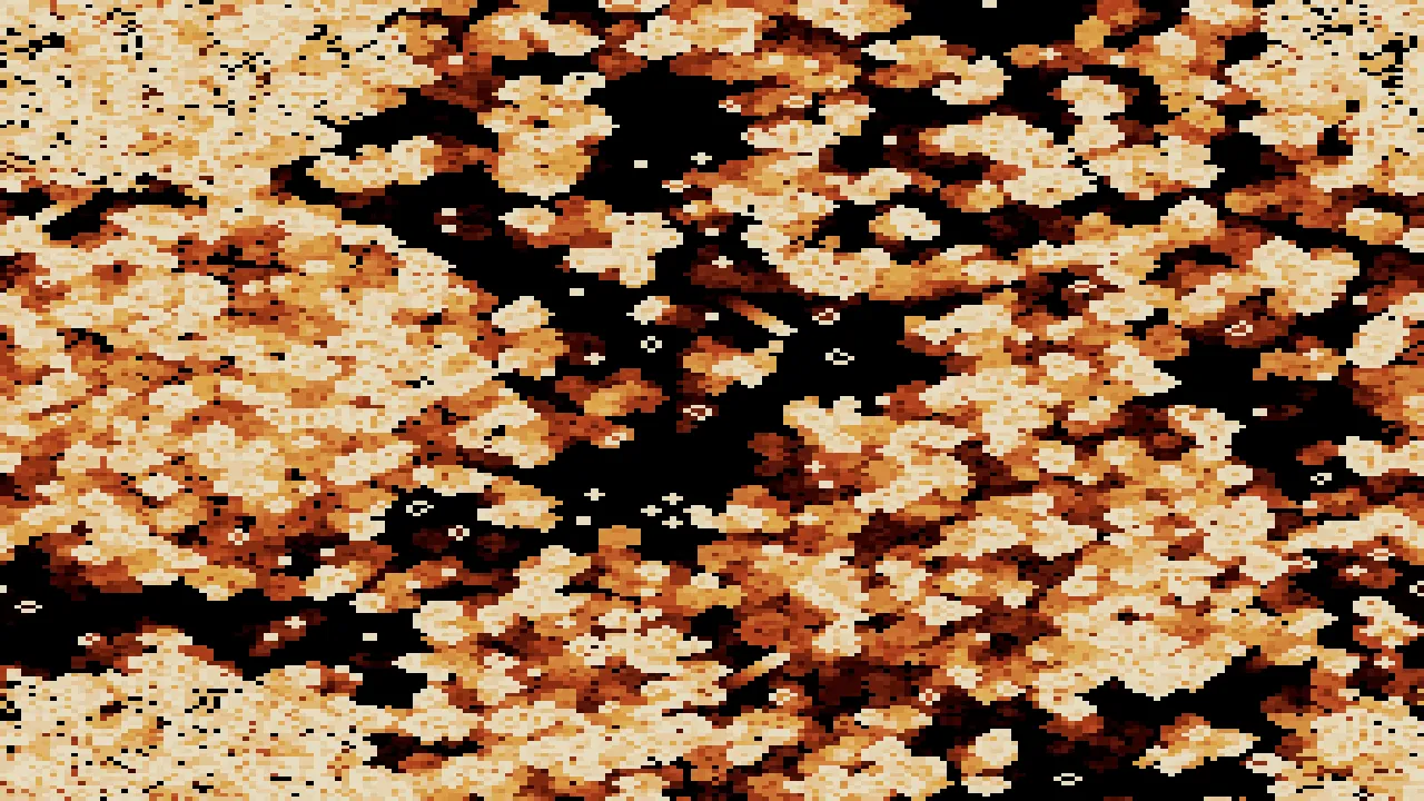
family = "life_like" — presets/cellular_ember_life.toml; the teaching preset is docs/examples/cellular/life_like.toml

A cellular automaton: a square grid of cells, every generation each cell deciding its next state from its neighbours’. The grid remembers — every cell carries how long ago it last changed — so a cell that has just died keeps glowing and fades out over trail generations. That wake is what turns a blinking checkerboard into something with history in it. step_rate is in generations per second, which makes it the lever for the music: bind it to the bass and the automaton runs faster when the bass does.

The picture above is Conway’s Life, birth = "8", survive = "12" — a rule written as two bitmasks over the neighbour counts, which the [cellular] table spells out. Left to itself Life settles into still lifes and blinkers, so reach for reseed — a disc of fresh cells on every rise, a beat or a latch — to keep it fed.

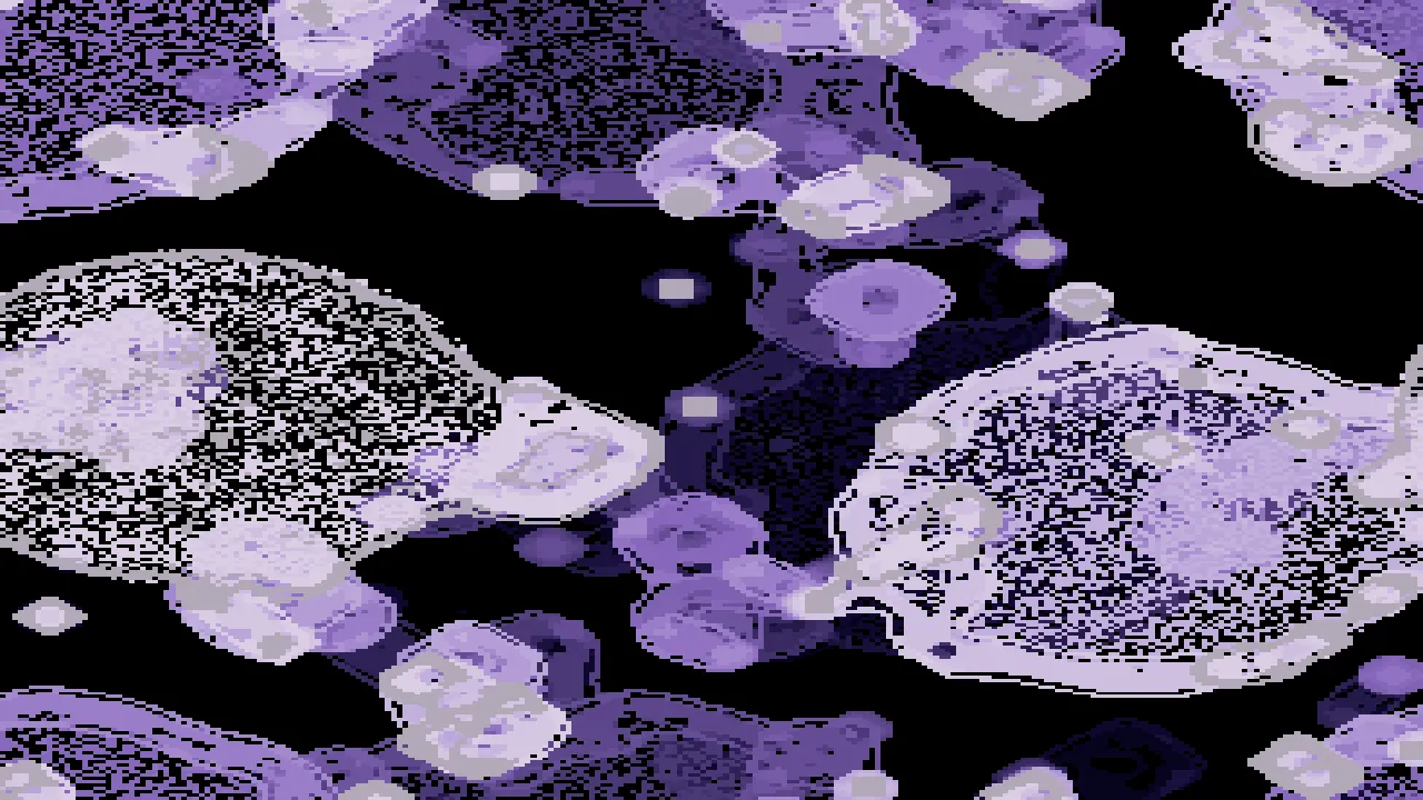
family = "larger_than_life" — presets/cellular_tide_bugs.toml; the teaching preset is docs/examples/cellular/larger_than_life.toml

Larger than Life reads a wide square of neighbours rather than eight, with birth and survival as ranges of how full it is. Above radius 1 its rules grow blobs and bugs that crawl, merge and split. Left alone they settle too, into still rings within a minute, so the preset pictured drops a fresh disc of soup on every hard onset and at least every five seconds; the speckled blobs above are those discs, organising.

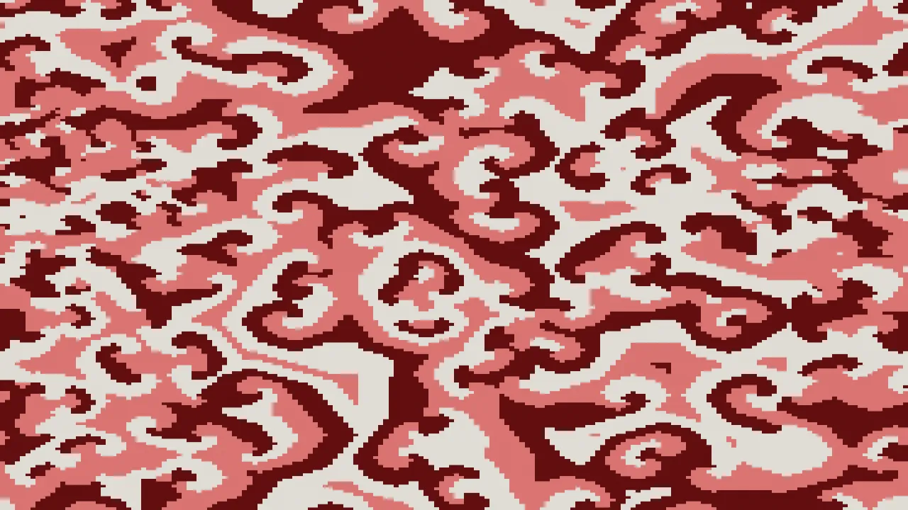
family = "cyclic" — presets/cellular_spiral_bloom.toml; the teaching preset is docs/examples/cellular/cyclic.toml

The cyclic automaton: every cell is one of states colours and advances to the next when enough neighbours already have. From noise it organizes itself, within a few hundred generations, into rotating spirals, and a cell’s colour is simply its place in the cycle laid round the palette.

Reach for this when the look is growth, colonies, waves or spirals that build up over time and hold their history. The grid is a count of cells, not a resolution — a larger grid draws every pattern smaller — and the families’ own parameters are in the [cellular] table.

plexus

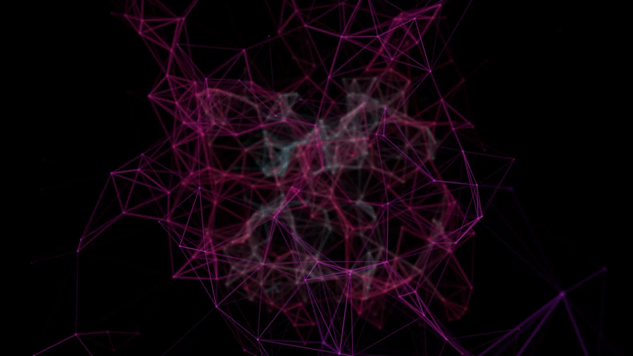
layout = "cloud" — the teaching preset docs/examples/plexus/cloud.toml; the shipped set has plexus_*.toml

A network in three dimensions: a few hundred points, each joined by a line to every other point closer than link_distance, seen through a camera that orbits the network’s centre. A line fades in as its two points drift together and out as they part, so the network rewires smoothly and never pops. link_distance is the main lever: a little longer and every point grows more links, and the network fills in. Bind it to the bass and the network knits together on every hit.

The camera is real, with a focal plane. focus places it in the network’s depth and aperture decides how strongly everything off it blurs, so one line can run sharp across the focal plane and soften toward both of its ends.

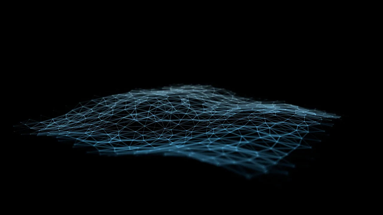
layout = "sheet" — the teaching preset docs/examples/plexus/sheet.toml

The sheet lays the points on a flat square instead and ripples it with a slow swell. Every point keeps its place in the grid, so the mesh moves like cloth rather than rearranging itself. Seen across at a grazing angle with the aperture open, the depth of field does the rest: a sharp band where the focal plane cuts the sheet, softness before and behind it.

Reach for this when the look is a network, a mesh or a constellation with depth to it, and the music should move the camera, the focus or how much of it is connected. Wide blur costs drawing time, so the quality tier caps it. The layouts and every structural key are in the [plexus] table.

waterfall

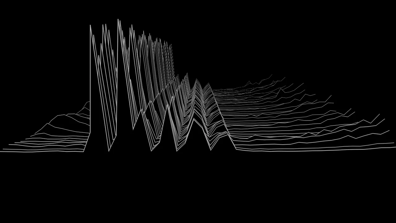
The shipped preset presets/waterfall_ridgeline.toml; the teaching preset docs/examples/waterfall/landscape.toml is the coloured version, seen from a little above

The spectrum’s recent past as terrain. Every fraction of a second the current band levels become a new row at the front, and the rows before it step back into the distance, so a sustained note leaves a ridge running away from you and a drum hit leaves a single crest that recedes. It is the spectrum system’s data with a memory, seen through the same camera as plexus: orbit it, look along it from low down, or put the focal plane on the front row and let the past blur away.

Reach for this when the look is the music’s shape over the last few seconds rather than this instant. rows and row_period set how much history there is, in the [waterfall] table.

voxel

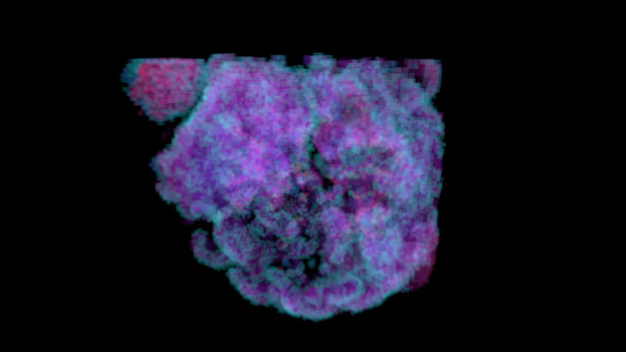
rules = ["pyroclastic"], density = "0.08" — the shipped preset presets/voxel_nebula.toml

A cellular automaton in three dimensions: a cube of cells, every generation each cell deciding its next state from how many of the cells around it are live, drawn as a glowing volume through the same camera as plexus. density decides how much the volume absorbs: at 0 every cell’s light adds up and the far side shows through the near one, and higher gives the cube a front surface that hides its inside.

A preset lists up to eight rules, from a named roster or written inline as two lists of neighbour counts, and the rule parameter picks one. Held on the bar, the automaton changes its mind at every bar line. Most 3D rules settle into a shape and hold it, so reseed on an onset is how the cube stays alive: each rise drops a ball of fresh cells that grows again.

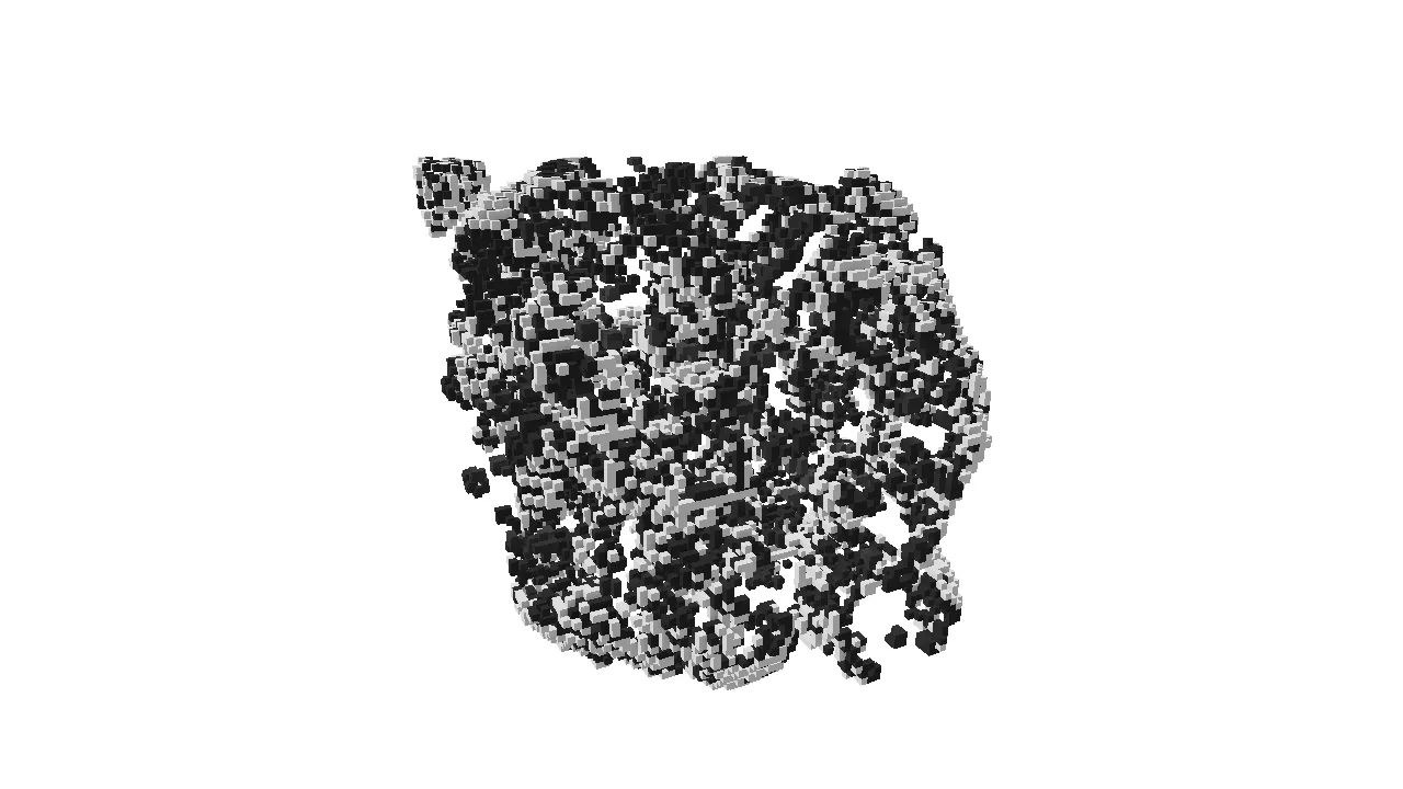
present = "solid", rules = ["pyroclastic"] — the teaching preset docs/examples/voxel/solid.toml, black on white, shipped as voxel_solid.toml; white on black is voxel_solid_dark.toml

present = "solid" draws every live cell as a lit cube instead of as light: one key light that turns with the camera, an ambient term, and an occlusion that darkens the creases where cubes meet, so the faces and corners of a structure read. The decaying cells in front of it still glow. Lift the ambient term toward 1 and the bloom over the faces, and the cubes read as lit from within instead: voxel_ember.toml is that look, and cut opens a solid structure along a plane to show its inside, as voxel_section.toml does.

Reach for this when the look is growth with depth to it: colonies, crystals, foam or clouds that build up inside a turning cube. The roster, the inline rule syntax and the tier caps are in the [voxel] table.

---

3. The three surfaces

Whatever system you pick, a preset touches three surfaces. Knowing which is which tells you which document to open.

Expressions — what moves. Every [params] value is a pure expression re-evaluated each frame against the current analysis frame. The vocabulary is the audio (bands, onset, beat, bar, tempo, novelty, the band array), a clock, arithmetic, comparisons, and a set of functions including clamp, select, sin, hash and noise. Expressions are pure — no state, no memory of the last frame — so anything that needs to persist is either a smoothing setting or a term built from a counter. The reference is Expression language, which also documents how a malformed expression is reported (the preset is rejected with a message; the app keeps the last good set and never crashes).

Structure — what is drawn. The structural tables — [curve], [generator], [particles], [spectrum] — are declarative and are read once, at load. They pick the curve family, the L-system’s axiom and rules, the attractor family and tuple, the spectrum’s element count and arrangement. Nothing here can be an expression, because changing it means rebuilding geometry rather than animating it. The reference is Parameter roster, which also carries every named parameter per system and the engine-wide stages every system accepts — background, trails, feedback, kaleidoscope, bloom, exposure and the ink remap.

Colour — how it is tinted. Palette-coloured systems address a shared lookup table rather than naming colours per element, so hue, saturation, color_span/hue_spread and color_center move a window over a gradient. You can name a built-in palette, write your own stops, quantize the result into hard bands, or cross-fade between two palettes. The reference is Colour and palettes.

There is a fourth, smaller surface worth knowing early: the [smoothing] table, which eases a parameter’s response over time and is the difference between an accent that snaps and glides and one that flickers. It is documented in Parameter roster, and step 4 of the walkthrough is a worked example of it.

---

4. Iterating

The loop is: point both the app and the capture tool at the same folder, edit, look.

Live, in the window. RLX_PRESET_DIR overrides the seeded per-user preset directory, and the app polls it every ~150 ms:

RLX_PRESET_DIR=./presets cargo run -p standalone --release

$env:RLX_PRESET_DIR = "./presets"; cargo run -p standalone --release   # PowerShell

Save a file and the change is on screen without a restart. Editing a file in presets/ without this is invisible to the app — seeding is write-if-absent, so a running frontend is reading its own seeded copy and will not see your edit.

Headless, as a picture. shot renders one preset with no window. It takes a single file directly, so an in-progress draft never has to enter the library:

cargo run -p standalone --example shot --release -- \
  --preset-file docs/examples/minimal.toml \
  --signal dynamic:110 --frame-at 300 --size 1280x720 --out draft.png

--signal dynamic:110 is the stimulus to use. It is the only synthesized kind with real rise and fall through the real analyzer; every other kind is a steady tone, and the --set path holds a constant value forever and cannot reach the band array at all. --frame-at <hop> picks one moment in that clip and writes it at full size. Every run prints the band levels the clip actually produced — min, mean and max per band — and those numbers, not --set magnitudes, are what a gain should be calibrated against.

To see the whole clip at once instead of one moment, swap --frame-at 300 for --strip 8 and you get a filmstrip. Headless capture and video is the reference for all of it.

---

5. Knowing it is good

Five gates in core/tests/ sweep every preset in presets/, and only one of them plays audio. That distinction is the most useful thing to know about them:

• reactivity drives real synthesized clips through the real FFT, band split and onset detector. It is the only gate that would notice a preset ignoring the music.
• sanity, animation, distinctness and golden construct an analysis frame directly, on purpose — their questions are about the frame, not the audio path. Each of them would pass a preset with every band binding deleted.

So a green suite means “this renders, moves, and is not a duplicate”. It does not mean “this reacts to music”, and it certainly does not mean “this looks good”. Headless capture and video has the full table of what each gate can and cannot see.

Two instruments are worth running by hand while you tune:

• shot --report prints per-preset reactivity, animation, coverage and transient columns, and accepts --preset-file, so you can measure a draft that has not shipped. The walkthrough uses it at every step.
• the band-level table that every --signal/--audio capture prints. If your gain was chosen against a --set magnitude it will be wrong by roughly an order of magnitude, and this table is how you find out.

One thing no instrument here can judge: whether the picture is good. That stays a human call.

---

6. Next

Tuning walkthrough takes one preset from constants to a finished look over five numbered steps, and shows the picture and the --report row that changed at each one — including the step where the numbers moved the wrong way.